Data structures and algorithms

Basic data structures

array: linear collection of fixed-size items stored contiguously in memory
- allows random access to elements (by index) and efficient iteration
  - time to access an element by index is $O (1)$
- arrays are fixed-size in memory, and increasing the array size requires copying the items to a new section of memory
  - dynamic array: array that doubles in size whenever it is filled
linked list: linear collection of items linked using pointers (so they don't need to be stored contiguously)
- single-linked list: each item only points to the next item
- double-linked list: each item also points to the previous item, so you can traverse the list in either direction
- pros:
  - space isn't preallocated, so it can hold as many items as you have memory
  - if you already have a pointer to the previous node, adding or removing items in the middle is more efficient than an array, since you don't need to move the items that come after
- cons:
  - no constant-time random access - finding elements is $O (n)$ since you need to traverse the list sequentially
  - requires extra space to store the pointers
stack: linear LIFO (Last In First Out) collection - insertion and removal are only allowed at one end of the list
- ex. function recursion, undo mechanisms
- commonly implemented with an array - each push/pop increments or decrements a counter so you know what the index of the last item is
queue: linear FIFO (First In First Out) collection - items are always inserted at one end and removed from the other end
- ex. handling incoming requests or messages
- commonly implemented with a linked list
hash table: mapping of keys to values, so you can easily find a specific value using its key
- the hash function maps data of arbitrary size (the values) to a fixed-size hash (the key)
  - lookups are $O (1)$ as long as there are no collisions, and space complexity is $O (n)$
- hash collisions are possible, but the hash should be designed so they're minimized
- common uses: data storage, caching, implementation of associative arrays (aka maps or dictionaries) and sets
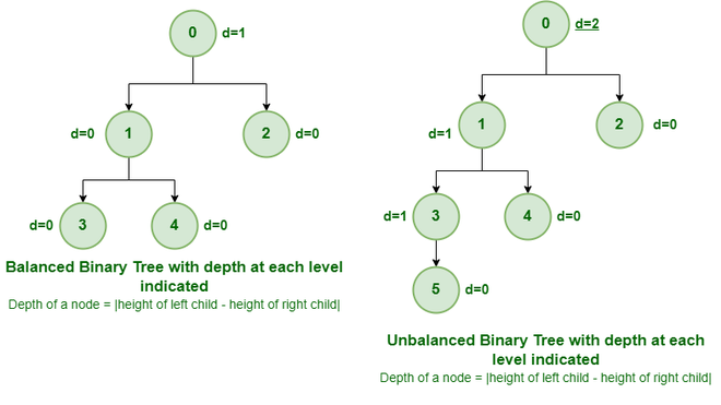
binary tree: tree where each node has at most two children
- the tree is represented in memory by a pointer to the topmost node, and each node contains its data and pointers to its left and right children
- balanced binary tree: tree where the height of the left and right subtrees for each node differ by no more than 1
- complete binary tree: binary tree where every level except possibly the last is completely filled, and all the nodes in the last level are as far left as possible
heap: a tree where values always increase or decrease as you move down the tree
- min heap: the root node has the smallest value, and every node is smaller than its children (the values increase as you go down)
- max heap: the root node has the largest value, and every node is larger than its children (the values decrease as you go down)
- binary heap: a heap that is also a complete binary tree
- common uses: sorting arrays, priority queues
binary search tree: a binary tree with the following properties:
- items on the left of a node are all less than that node's value
- items on the right of a node are all greater than that node's value
- there are no duplicate nodes
- efficient for searching ( $O (l o g n)$ ) because you can remove ~50% of the nodes with every comparison
graph: a fixed set of nodes or vertices connected by edges
- common uses: representing networks (such as social media networks, or paths through a city)

Sorting algorithms

Bubble sort: keep iterating two at a time, swapping the items if they're in the wrong order, until sorted
- simple, but not efficient
- best case $O (n)$ (data already sorted), worst case $O (n^{2})$ (data in the opposite order)
Selection sort: iterate through, find the smallest item and move it to the front of the list, and repeat
- best case $O (n)$ , worst case $O (n^{2})$ , but fewer swaps than Bubble Sort
Insertion sort: iterate through, and for each item, move its neighbors in front or behind depending on whether they're greater or less than it
- best case $O (n)$ , worst case $O (n^{2})$
QuickSort: Choose a pivot (usually in the center) and split the array into two sub-arrays around the pivot. Create two pointers, one at the start of the left subarray and one at the end of the right subarray. Iterate toward the pivot until you find a pair of numbers where the left one is larger than the pivot and the right one is smaller than the pivot. Swap those two numbers. Once both pointers reach the pivot, repeat QuickSort on the subarrays.
- used if the array is small or there are few elements left to sort
- best and average case $O (n l o g n)$ , worst case $O (n^{2})$ (if the smallest or largest element is chosen as the pivot)
MergeSort: break the array into pieces one wide, then merge the pieces into two wide so they're in the correct order, then sort the two wide pieces and merge those in the correct order, repeat
- worst and average case $O (n l o g n)$
bucket sort: divide the array into buckets (stacks) by ranges, sort each bucket with any sorting algorithm or recursive BucketSort, then merge the buckets in order
- used with floating point numbers or input that is uniformly distributed over a range
- worst case, elements are all placed in one bucket, so complexity is whatever sorting algorithm is used on that bucket
- average case $O (n)$ if elements are randomly distributed
- best case $O (n + k)$ if the elements are uniformly distributed, where $k$ is the number of buckets
heap sort: place the elements in a heap (a tree where the root has the largest value and children are always smaller, or vice versa), then take the root (which will be the largest or smallest of the remaining values), re-heapify the tree, and repeat
- like selection sort, but instead of a linear-time scan of the unsorted data, you just maintain it in a heap
- no additional space required
- great if you only need the smallest or largest of the remaining items, ex. in a priority queue
- in practice, usually slower than quicksort, but implementation is simple and worst-case is better
- not a stable sort
- $O (n l o g n)$ for best, worst, and average case

Tree search types

breadth-first search:
- starting at the root, explore each level fully before moving on to the next level
- implemented with a queue, to keep track of child nodes that were found but not visited yet
depth-first search:
- starting at the root, explore as long as possible along the leftmost branch before backtracking
- implemented with a stack, to keep track of nodes discovered along the branch - stack lets you pop the nodes to backtrack once you reach the end of the current branch
- if the tree has an infinite branch, DFS is not guaranteed to find the solution

Big O notation

LeetCode course

can be used to measure time or space complexity
- time complexity: as the input size grows, how does the elapsed time grow?
- space complexity: as the input size grows, how much more memory is required?
usually consider three cases: best case, average case, and worst case
- for most algorithms these are equal, but if you only use one it should be the worst case
ignore constants: $O (5000 n) = O (n)$
imagine all variables trending to infinity: $O (2^{n} + n^{2} - 500 n) = O (2^{n})$ , because as $n$ grows, $2^{n}$ becomes large enough to make the other two terms irrelevant
- similarly, $O (n + 5000) = O (n)$

Time complexity examples

$O (1)$ : uses the same resources no matter the input size

print(input)

for i in range(5000):
    print(input) # O(5000) = O(1)

$O (n)$ : complexity scales linearly with the input size

for i in input:
    print(input)
# or
for i in input:
    for j in range(5000):
        print(input)
        # even though there are nested loops, the inner loop runs the same
        # number of times for each item in input, and O(5000n) === O(n)

$O (n^{2})$ :

for i in input:
    for j in input:
        print(i * j)
        # the inner loop runs n times each time the outer loop runs,
        # so O(n * n) = O(n^2)

$O (n + m)$ :

for i in input1:
    print(i)

for i in input1:
    print i

for i in input2:
    print i

# O(2n + m) = O(n + m)

$O (n^{2})$ : (partial series explanation)

for (let i = 0; i < input.length; i++) {
    for (let j = i; j < input.length; j++) {
        console.log(input[i] + input[j])
    }
}

// the inner loop depends on what iteration the outer loop is on
// on the first outer loop iteration, the inner loop runs n times
// on the second outer loop iteration, the inner loop runs n - 1 times, etc.
// therefore, the total number of iterations is 1 + 2 + 3 + ... + n,
// which equals n(n + 1)/2 = (n^2 + n)/2 = O(n^2)
// the addition in the numerator and constant in the denominator are ignored

Python equivalent:

for i in range(len(input)):
    for j in range(i, len(input)):
        print(i, j, input[i], input[j], input[i] + input[j])

Logarithmic complexity

Logarithms are the inverse of exponents, so logarithmic time ( $O (l o g n)$ ) is extremely fast
- $O (l o g n)$ means the input is being reduced by a percentage at every step
  - ex. binary search - at each step the input is reduced by 50%
- $O (n * l o g n)$ is a common time complexity for efficient sorting algorithms

Two Pointers

technique for solving array and string problems
uses two indexes that move along the iterable, often from opposite ends
will always run in $O (n)$ time, as long as the work in each iteration is $O (1)$
all of the examples below have $O (1)$ space complexity, since no variables are created within the loops
example: determine if a string is a palindrome

def check_palindrome(string):
    i, j = 0, len(string) - 1
    while i < j:
        if string[i] != string[j]:
            return False
        i += 1
        j -= 1
    return True

print(check_palindrome("racecar"))  # True
print(check_palindrome("banana"))  # False
print(check_palindrome("amanaplanacanalpanama"))  # True

given a sorted array of unique integers and a target integer, see if any pair of numbers in the array sum to the target
- brute force solution would be to check every pair in the array, which would be $O (n^{2})$
- but since the array is sorted, we can use two pointers to do it in $O (n)$

def can_reach_target(nums, target):
    i, j = 0, len(nums) - 1
    while i < j:
        sum = nums[i] + nums[j]
        if sum == target:
            print(nums[i], nums[j])
            return True
        elif sum < target:
            # the sum needs to be bigger, so move the left pointer up
            i += 1
        elif sum > target:
            # the sum needs to be smaller, move the right pointer down
            j -= 1
    return False

print(can_reach_target([1, 2, 4, 6, 8, 9, 14, 15], 13))  # 9, 4

not all two pointers problems iterate one array - they can also iterate along two arrays (not necessarily at the same rate)
ex. given two sorted integer arrays, return a new array that combines both of them and is also sorted
- naive solution would be to combine the arrays and then sort the result, which will be $O (n * l o g n)$ (the cost of the sorting algorithm)
- but since the arrays are sorted, we can do it with two pointers in $O (n)$

def combine(nums1: list[int], nums2: list[int]):
    i = j = 0
    result = []
    while i < len(nums1) and j < len(nums2):
        # on each iteration, take the smaller of the two current numbers
        if nums1[i] < nums2[j]:
            result.append(nums1[i])
            i += 1
        else:
            result.append(nums2[j])
            j += 1

    # append the rest of the nums
    while i < len(nums1):
        result.append(nums1[i])
        i += 1
    while j < len(nums2):
        result.append(nums2[j])
        j += 1

    assert len(result) == len(nums1) + len(nums2)
    return result

print(combine([5, 9, 20, 48, 60, 201], [19, 38, 95]))
print(combine([19, 38, 95], [5, 9, 20, 48, 60, 201]))

given two strings, check if the first is a subsequence of the second
- characters in a subsequence don't have to be contiguous - ex. ace is a subsequence of abcde

def is_subsequence(sub: str, full: str):
    i = j = 0
    while i < len(sub) and j < len(full):
        # step through the full string, and increment i each time we find a
        # character of the subsequence string
        if sub[i] == full[j]:
            i += 1
        j += 1
    # we know it's a subsequence if we found all the characters
    return i == len(sub)

print(is_subsequence("ace", "abcde"))  # true
print(is_subsequence("adb", "abcde"))  # false

Sliding Window

another common technique for array and string problems, where you look for valid subarrays
- implemented with #Two Pointers (left and right) that mark the start and end indices (inclusive) of the subarray
problems that can be solved efficiently with sliding window have two criteria:
- a constraint metric - some attribute of a subarray (the sum, number of unique elements, etc)
  - the constraint metric has to meet a numeric restriction for the subarray to be considered valid - ex. sum <= 10
- the problem asks you to find subarrays in some way - for example, the number of valid subarrays, or the best subarray as defined by a given criteria (such as the longest valid subarray)
process:
- start with left = right = 0 - in other words, the window covers just the first element
- use a for loop to increment right, because we know we want the window to "check" every item
- while the subarray is invalid, shrink the window by incrementing left until it becomes valid again

# pseudocode
left = 0
for right in range(len(arr)):
    # add the element at arr[right] to the window
    while WINDOW_IS_INVALID:
        # remove the element at arr[left] from the window
        left += 1
    # update the answer if necessary - remember the current state of the
    # window may not "beat" the current answer
return answer

if the logic for each window is $O (1)$ , then the algorithm runs in $O (n)$
- the left and right pointers can each move a maximum of $n$ times, so the complexity is $O (2 n) = O (n)$
  - right always moves $n$ times because of the for loop
  - left can move a maximum of $n$ times, because at that point $l e f t = r i g h t = n$
- looking at every possible subarray would be at least $O (n^{2})$ , much slower
ex. find the length of the longest subarray with a sum <= the given number k
- constraint metric: the sum of the window

def longest_sub(nums: list[int], k: int):
    left = 0
    sum = 0
    # we use a separate answer variable because the state of `left` and
    # `right` at the end of the for loop may not be the correct solution
    answer = 0
    for right in range(len(nums)):
        sum += nums[right]
        while sum > k:
            sum -= nums[left]
            left += 1
        # only overwrite answer if the current subarray is larger than the
        # previous largest
        answer = max(answer, right - left + 1)
    return answer

print(longest_sub([3, 2, 1, 3, 1, 1], 5))  # 3
print(longest_sub([1, 2, 3, 4, 5, 50000], 9999))  # 5
print(longest_sub([10, 20, 30, 40, 50], 1)) # 0

ex. Given a binary string (made up of only 0s and 1s), you're allowed to choose up to one 0 and flip it to a 1. What is the longest possible substring containing only 1s?
- another way to look at this problem is, "what is the longest possible substring that contains at most one 0?"

def longest_ones(str: str):
	left = 0
	zero_count = 0
	answer = 0
	for right in range(len(str)):
		if str[right] == '0': zero_count += 1
		while zero_count > 1:
			if str[left] == '0': zero_count -= 1
			left += 1
		answer = max(answer, right - left + 1)
	return answer

print(longest_ones('1101100111')) # 5

if a problem asks for the number of subarrays that fit a constraint, add up the number of valid subarrays ending at each index (each value of right)
- if your current window is valid, the number of subarrays ending at right will be the same as the window size, which is $r i g h t - l e f t + 1$ - (left, right), (left + 1, right), etc. up to (right, right)
ex. Given an array of positive integers and an integer k, find the number of subarrays where the product of all the elements is less than k

def count_valid_sublists(nums: list[int], limit: int):
    if limit <= 1:
        return 0

    left = 0
    product = 1
    count = 0
    for right in range(len(nums)):
        product *= nums[right]
        while product >= limit:
            product /= nums[left]
            left += 1
        count += right - left + 1
    return count

print(count_valid_sublists([10, 5, 2, 6], 100))  # 8

if a problem asks for a fixed window size, start by finding the answer for the first window (0, k -1), then slide the window along one at a time and keep checking if the new answer beats the current one
ex. given an integer array and an integer k, find the sum of the subarray of length k that has the largest sum

def largest_sum(nums: list[int], k: int):
    sum = 0
    for i in range(k):
        # get the sum of the numbers in the initial window
        sum += nums[i]
    answer = sum

    for i in range(k, len(nums)):
        # add the upcoming number and subtract the one leaving the window
        sum += nums[i] - nums[i - k]
        answer = max(answer, sum)
    return answer

print(largest_sum([3, -1, 4, 12, -8, 5, 6], 4))  # 8

Dynamic programming

LeetCode course

can be used to solve problems that fulfill both these criteria:
- can be broken down into overlapping subproblems: smaller versions of the original problem that are reused multiple times
  - compare to a greedy problem, where you make the locally optimal choice at each step, but don't need to consider previous steps
- has an optimal substructure: by finding optimal solutions to the subproblems, you form an optimal solution to the original problem
because subproblems overlap, DP solutions aren't easy to parallelize, unlike divide and conquer solutions
example: calculate the Fibonacci number F(n) for a given value of n
- the subproblems are F(n-1) and F(n-2) - they overlap because to find both, you'll need F(n-3)
- the original problem has an optimal substructure, because if you solve F(n-1) and F(n-2) you find the solution to F(n)
two ways to solve a DP problem:
- bottom-up (tabulation): start at the base cases and work up using iteration
  - for the example, start with F(0) = 0 and F(1) = 1, then calculate F(2), F(3), etc up to F(n)
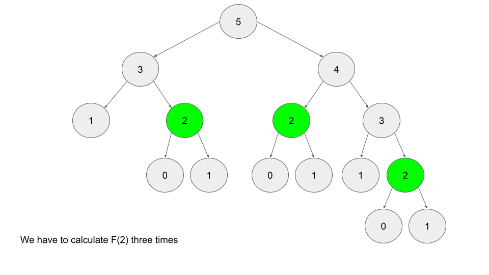
- top-down (memoization): solve the subproblems using recursion from the top down, and save (memoize) the results of each subproblem so you don't need to repeat calculations
  - for example, to calculate F(5) you need to calculate F(2) three times, unless you save the result (typically in a hashmap)
- bottom-up tends to be faster, but top-down is easier to write (because the order of solving subproblems doesn't matter)
to identify DP problems:
- typically ask for an optimum value (minimum, maximum, longest, etc), or whether it's possible to reach a certain point
- future steps depend on previous steps
another example, House Robber:

You are a professional robber planning to rob houses along a street. Each house has a certain amount of money stashed, the only constraint stopping you from robbing each of them is that adjacent houses have security systems connected and it will automatically contact the police if two adjacent houses were broken into on the same night.

Given an integer array nums representing the amount of money of each house, return the maximum amount of money you can rob tonight without alerting the police.

for the case [2, 7, 9, 3, 1], the optimal solution is [2, 9, 1]
the first decision to make is whether to rob the first or second house, but this affects which options are available in future decisions
- a greedy solution would choose to rob the second house first (since 7 > 2), but this prevents robbing the third house - decisions affect other decisions